set.seed(6556)
x <- 1:20
y <- x + rnorm(20, sd=3)  # y is correlated with x
z <- sample(1:20,20)/2 + rnorm(20, sd=5)
df <- data.frame(x,y,z)15 Correlations and linear regression
Correlation
We say that two variables are correlated when a change in one is associated with a change in the other.
To visualize this, generate some synthetic data with random noise and correlation.
options(repr.plot.width=8, repr.plot.height=3)
par(mfrow=c(1,3))
plot(df$x, df$y)
plot(df$x, df$z)
plot(df$y, df$z)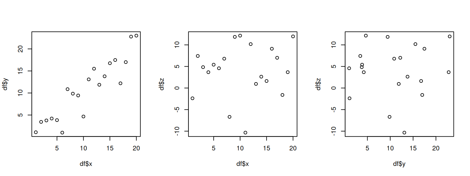
We can see that x and y are correlated positively: When one increases, the other increases, too. On the other hand, z does not seem not correlated with the rest.
Let’s check this intuition by calculating the Pearson correlation coefficient. This coeffiecient has values between -1 and 1, 1 indicating perfect positive correlation, an 0 indicating no correlation.
cor(df, method="pearson") x y z
x 1.0000000 0.91448499 0.11100764
y 0.9144850 1.00000000 0.04973288
z 0.1110076 0.04973288 1.00000000The correlation coefficient between x and y is close to 1, and that between z and the others is small.
However, these results might be due to luck, resulting from the finite number of data we got.
The correlation test gives us a confidence interval about this result.
cor.test(df$x, df$y, method="pearson")
    Pearson's product-moment correlation

data:  df$x and df$y
t = 9.5888, df = 18, p-value = 1.697e-08
alternative hypothesis: true correlation is not equal to 0
95 percent confidence interval:
 0.7927889 0.9660614
sample estimates:
     cor
0.914485 cor.test(df$x, df$z, method="pearson")
    Pearson's product-moment correlation

data:  df$x and df$z
t = 0.47389, df = 18, p-value = 0.6413
alternative hypothesis: true correlation is not equal to 0
95 percent confidence interval:
 -0.3486394  0.5276105
sample estimates:
      cor
0.1110076
Let’s apply this to a data set we have used before, the height and weight data for men and women.
url <- "https://raw.githubusercontent.com/johnmyleswhite/ML_for_Hackers/refs/heads/master/02-Exploration/data/01_heights_weights_genders.csv"
heights_weights_gender <- read.table(url, header=T, sep=",")
men <- heights_weights_gender$Gender == "Male"
men_heights <- heights_weights_gender[["Height"]][men]
men_weights <- heights_weights_gender[["Weight"]][men]
women <- heights_weights_gender$Gender == "Female"
women_heights <- heights_weights_gender[["Height"]][women]
women_weights <- heights_weights_gender[["Weight"]][women]
plot(men_heights, men_weights)
cor.test(men_heights,men_weights)
    Pearson's product-moment correlation

data:  men_heights and men_weights
t = 120.75, df = 4998, p-value < 2.2e-16
alternative hypothesis: true correlation is not equal to 0
95 percent confidence interval:
 0.8557296 0.8698894
sample estimates:
      cor
0.8629788 cor.test(women_heights,women_weights)
    Pearson's product-moment correlation

data:  women_heights and women_weights
t = 113.88, df = 4998, p-value < 2.2e-16
alternative hypothesis: true correlation is not equal to 0
95 percent confidence interval:
 0.8417121 0.8571417
sample estimates:
      cor
0.8496086
Correlation does not always mean causation
If A and B are correlated, this might mean there is a causal link between them, but this correlation can be due to other factors. It can be due to chance, even.
A causes B, e.g. rain and crop growth.
A and B influence each other; e.g., rain causes tree growth, and evaporation from large forests cause rain.
However, correlation can also exist without causation.
Both A and B are may be influenced by another factor
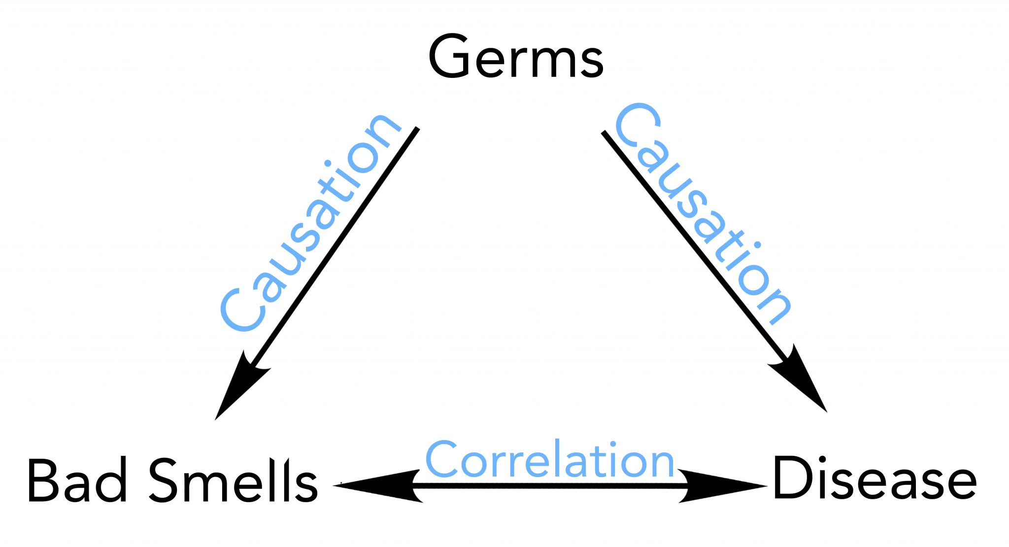
Pure luck, no causation.
 (Source)
The Anscombe Quartet
Correlation is a summary statistic. It can hide important features of data.
A famous example is the Anscombe data set, which illustrates that very different data can lead to the same correlation coefficient.
anscombe x1 x2 x3 x4 y1 y2 y3 y4
1 10 10 10 8 8.04 9.14 7.46 6.58
2 8 8 8 8 6.95 8.14 6.77 5.76
3 13 13 13 8 7.58 8.74 12.74 7.71
4 9 9 9 8 8.81 8.77 7.11 8.84
5 11 11 11 8 8.33 9.26 7.81 8.47
6 14 14 14 8 9.96 8.10 8.84 7.04
7 6 6 6 8 7.24 6.13 6.08 5.25
8 4 4 4 19 4.26 3.10 5.39 12.50
9 12 12 12 8 10.84 9.13 8.15 5.56
10 7 7 7 8 4.82 7.26 6.42 7.91
11 5 5 5 8 5.68 4.74 5.73 6.89options(repr.plot.width=8, repr.plot.height=8)
par(mfrow = c(2,2))
plot(anscombe$x1, anscombe$y1)
plot(anscombe$x2, anscombe$y2)
plot(anscombe$x3, anscombe$y3)
plot(anscombe$x4, anscombe$y4,xlim=c(4,20))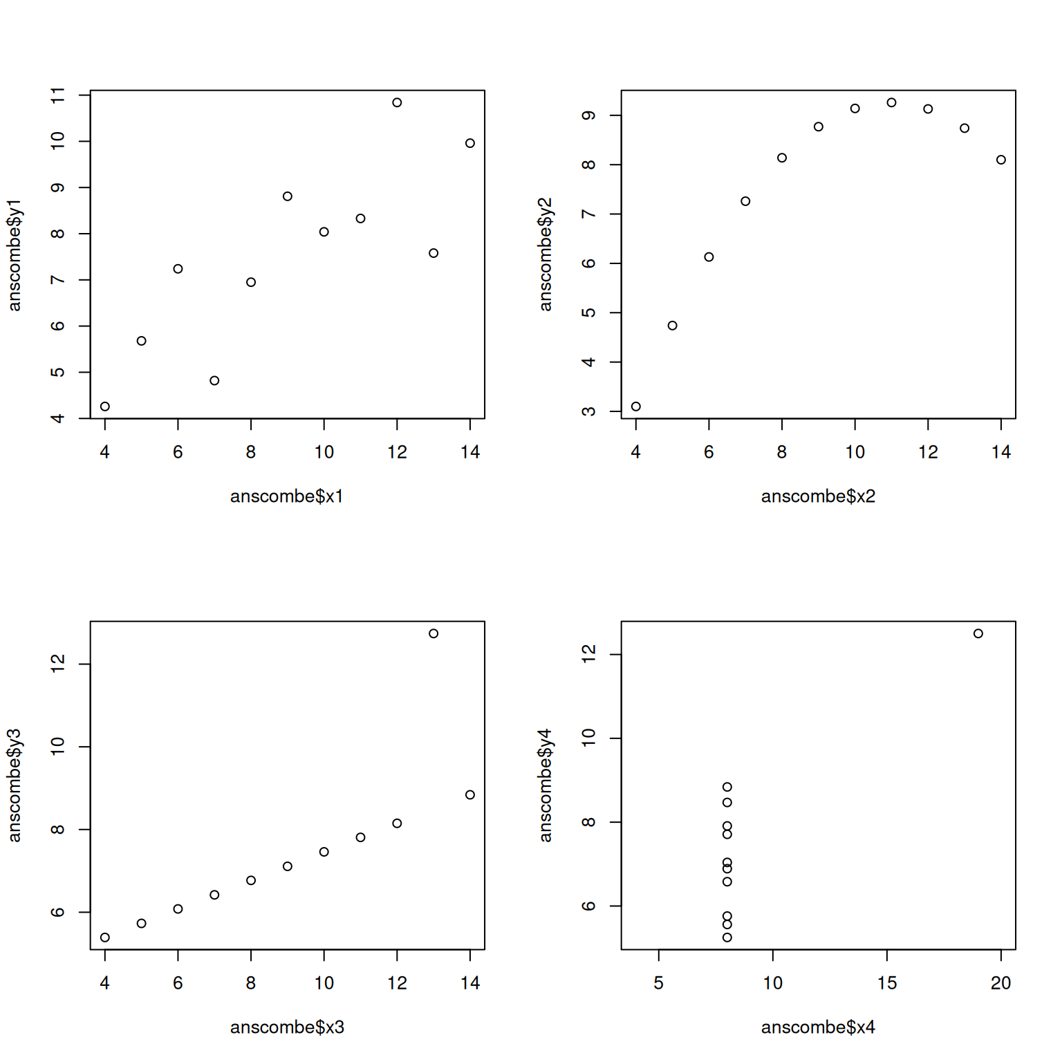
Despite fundamental differences, the correlation coefficient for each pair of variables is the same.
cor(anscombe$x1, anscombe$y1)[1] 0.8164205cor(anscombe$x2, anscombe$y2)[1] 0.8162365cor(anscombe$x3, anscombe$y3)[1] 0.8162867cor(anscombe$x4, anscombe$y4)[1] 0.8165214Linear regression
When we discover a correlation between two variables \(x\) and \(y\), we may want to find out a formula for the relation between them. That way, we can predict the outcome of unobserved input values.
We assume a linear relationship \(y=ax+b\) between variables \(x\) and \(y\). Then, given the observations \((x_1,y_1),\ldots,(x_n,y_n)\), the statistical procedure to determine the coefficients \(a\) and \(b\) is called linear regression.
Once we have some estimates \(\hat{a}\) and \(\hat{b}\) for the parameters, when we get a new input value \(x\), we can predict the outcome as \(y=\hat{a}x + \hat{b}\).
Let’s create a synthetic data set again.
set.seed(1235)
x <- 1:10 + rnorm(10,sd=2)
y <- x + rnorm(10, sd=3)
df <- data.frame(x,y)
df
x y
1 -0.3959759 -3.217074
2 -0.5697077 2.685184
3 4.9799180 2.729447
4 4.2235517 2.958473
5 5.2284153 2.758888
6 9.3963930 10.634494
7 7.0956912 8.935584
8 9.3097248 7.947907
9 11.7305673 9.731882
10 10.8051459 11.754786plot(x,y)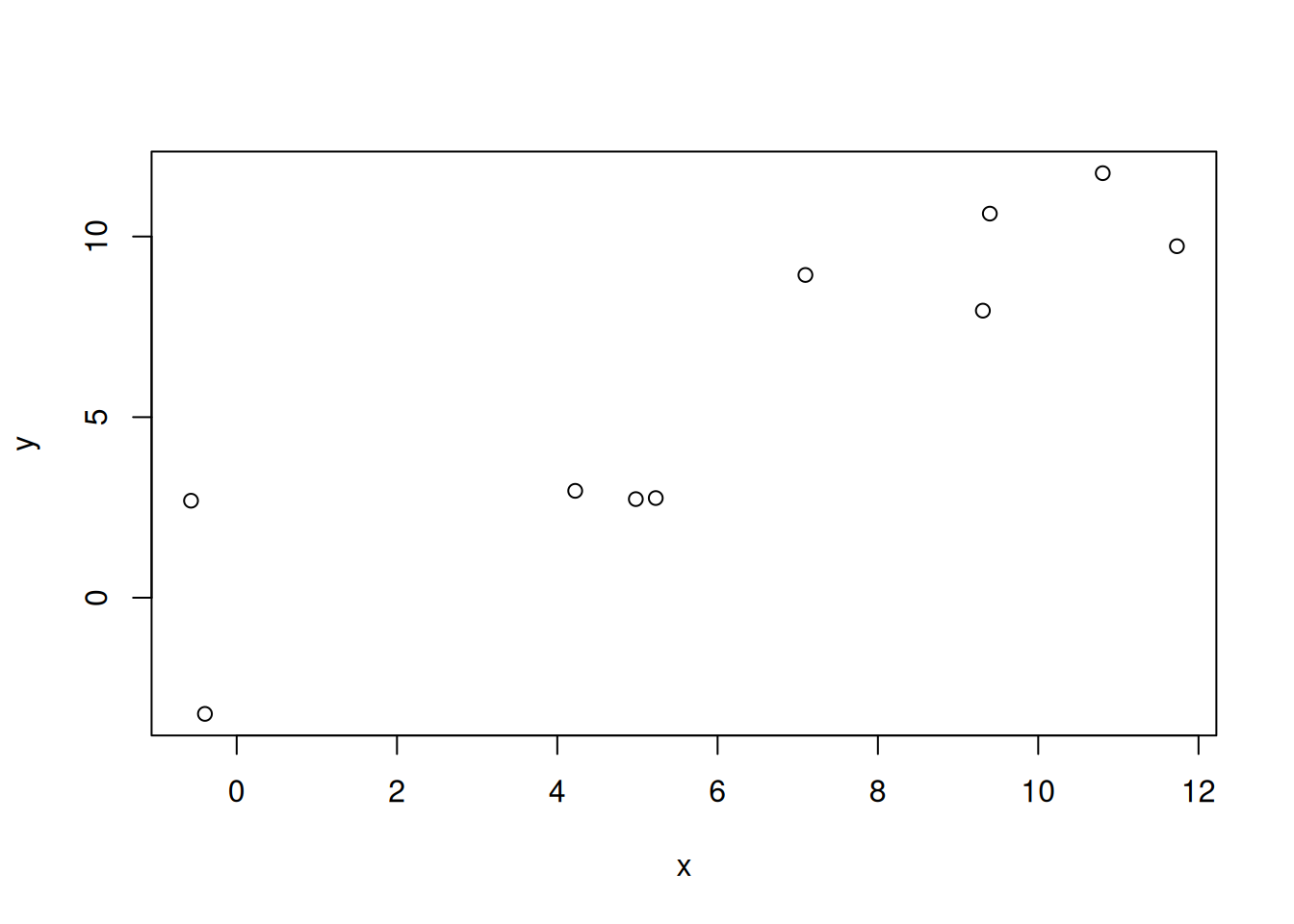
Our purpose is to draw a line such that the distances between given points and the line are minimized. R provides a function lm() (for “linear model”) that performs this task.
linmodel <- lm(y~x, data=df)
linmodel
Call:
lm(formula = y ~ x, data = df)

Coefficients:
(Intercept)            x
    -0.4448       0.9929
We see a nonzero intercept, even though we expect zero. Is this reliable? To understand this, we look at statistical information about the regression.
summary(linmodel)
Call:
lm(formula = y ~ x, data = df)

Residuals:
    Min      1Q  Median      3Q     Max
-2.3791 -1.6957 -0.8209  1.6796  3.6956

Coefficients:
            Estimate Std. Error t value Pr(>|t|)
(Intercept)  -0.4448     1.2884  -0.345 0.738831
x             0.9929     0.1737   5.716 0.000446 ***
---
Signif. codes:  0 '***' 0.001 '**' 0.01 '*' 0.05 '.' 0.1 ' ' 1

Residual standard error: 2.253 on 8 degrees of freedom
Multiple R-squared:  0.8033,    Adjusted R-squared:  0.7787
F-statistic: 32.67 on 1 and 8 DF,  p-value: 0.000446
The output tells us that the intercept value is not statistically significant.
A more concrete piece of information is the confidence interval.
confint(linmodel) 2.5 % 97.5 %
(Intercept) -3.4158320 2.526273
x 0.5923686 1.393511A detailed understanding of this quantity should be delegated to a statistics class. for us, it is sufficient that the confidence interval for the intercept includes the value zero. This indicates that we have no reason to think that the intercept is nonzero.
The regression model can be plotted with the abline() function.
plot(x,y)
abline(linmodel, col="red")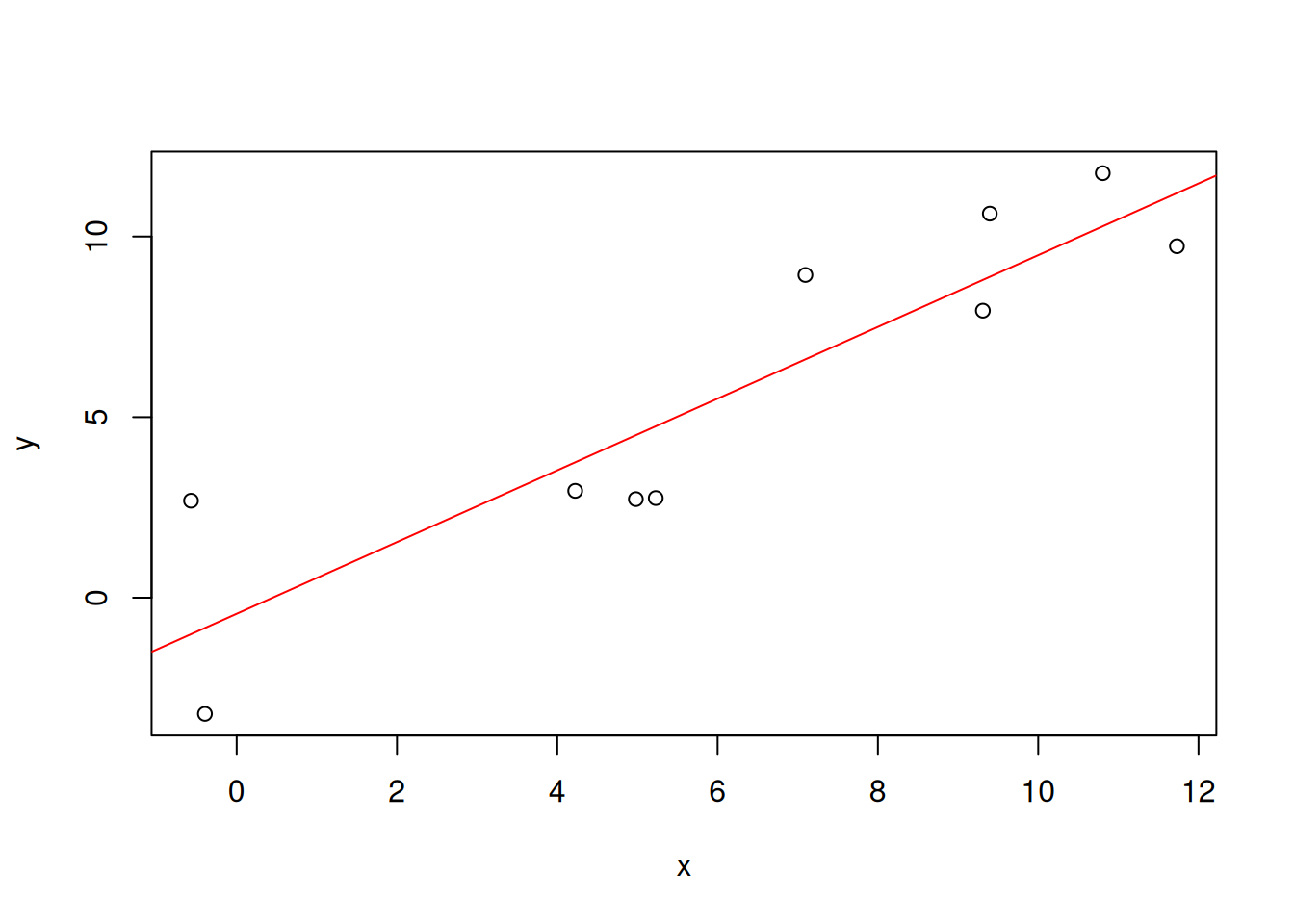
Let’s make a prediction for \(x=25,26,\ldots,30\).
newx <- 25:30
predict.lm(linmodel, data.frame(x=newx))
1 2 3 4 5 6
24.37871 25.37165 26.36459 27.35753 28.35047 29.34341 Linear regression of height and weight data
Let’s go back to the height and weight data for men and women. We have already established that there is a strong correlation between these variables, within each gender.
df <- data.frame(men_heights,men_weights,women_heights,women_weights)
head(df)
men_heights men_weights women_heights women_weights
1 73.84702 241.8936 58.91073 102.0883
2 68.78190 162.3105 65.23001 141.3058
3 74.11011 212.7409 63.36900 131.0414
4 71.73098 220.0425 64.48000 128.1715
5 69.88180 206.3498 61.79310 129.7814
6 67.25302 152.2122 65.96802 156.8021The next question is, how much does the weight increase for every inch of height?
Let’s train a linear model for each gender. The coefficient (slope) is the answer to this question.
men_hw_model <- lm("men_weights ~ men_heights",
  data=df)
women_hw_model <- lm("women_weights ~ women_heights",
  data=df)

men_hw_model
Call:
lm(formula = "men_weights ~ men_heights", data = df)

Coefficients:
(Intercept)  men_heights
   -224.499        5.962
So, for every additional inch in height, a man’s weight increases, on average, by about 6 lbs.
plot(men_heights,men_weights)
abline(men_hw_model,col="red")
Repeating the same for women, we see almost the same value for the coefficient.
women_hw_model
Call:
lm(formula = "women_weights ~ women_heights", data = df)

Coefficients:
  (Intercept)  women_heights
-246.013 5.994 plot(women_heights,women_weights)
abline(women_hw_model,col="red")
The two linear models mainly differ in their intercepts.
Linear regression with multiple variables
Our linear model can involve two independent variables: \[y = a_0 + a_1x_1 + a_2 x_2\]
Let’s generate some synthetic data by adding random noise around \(y = x_1+2x_2\):
# generate synthetic data
set.seed(1234)
x1 <- sample(1:20,20) + rnorm(20,sd=2)
x2 <- sample(1:20,20)/2 + rnorm(20, sd=5)

y <- 0 + 1*x1 + 2*x2 + rnorm(10, sd=3)
df <- data.frame(x1,x2,y)
df
x1 x2 y
1 12.625346 -2.2599294 12.208969
2 3.745128 5.8808594 19.495541
3 12.036633 7.5157502 28.077552
4 16.410487 -4.0301563 8.370853
5 7.705962 5.0896204 16.518797
6 20.736362 1.9555519 23.547894
7 6.751271 -2.0748100 4.546511
8 4.620524 0.6884524 12.208242
9 2.010014 7.3152791 16.180377
10 6.924739 14.7390874 32.230811
11 15.447952 3.1332329 25.817899
12 9.006522 14.0295481 41.054313
13 11.022790 -4.7890427 2.454123
14 20.019720 6.7829423 33.606283
15 14.356543 22.2449554 57.480047
16 10.059126 2.3261981 13.611950
17 13.540943 -2.8481679 9.789467
18 -3.408696 5.4619762 13.726069
19 19.086346 10.8854222 40.396995
20 3.042854 3.3069613 5.484674plot(df)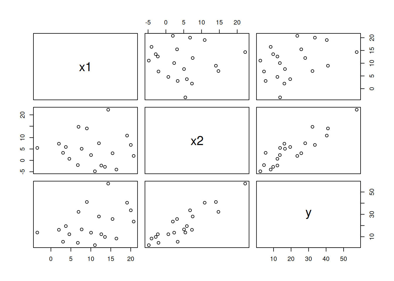
Using the same formula system, we can simply extend the regression to two independent variables:
linmodel2 <- lm(y~x1+x2, data=df)
linmodel2
Call:
lm(formula = y ~ x1 + x2, data = df)

Coefficients:
(Intercept)           x1           x2
2.7540 0.8876 1.8784 confint(linmodel2) 2.5 % 97.5 %
(Intercept) -0.1173064 5.625245
x1 0.6656861 1.109491
x2 1.6702903 2.086563Linear regression with polynomials
The name “linear regression” might suggest that it cannot be used for fitting nonlinear models, such as polynomials \(y=a_0 + a_1x + a_2x^2 + a_3x^3+...\)
However, by treating different powers as independent variables, we can treat this as a multiple regression model.
Consider the following synthetic data:
set.seed(8764)
x <- 0:19
y <- -0.1*x^2 + 2*x + 1 + rnorm(20, sd=2)
plot(x,y)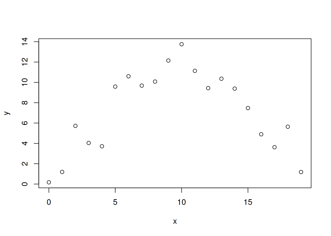
This model is obviously not linear in \(x\). To apply linear regression, create new variables: \(x_1 := x\) and \(x_2 := x^2\). Then we can set up a linear model with two independent variables as before.
x1 <- x
x2 <- x^2
quadmodel <- lm(y~x1+x2, data=data.frame(x1,x2,y))
quadmodel
Call:
lm(formula = y ~ x1 + x2, data = data.frame(x1, x2, y))

Coefficients:
(Intercept)           x1           x2
    -0.4860       2.3705      -0.1202
The estimated model is \(\hat{y} = -0.1202x^2 + 2.3705x-0.4860\), while the truth was \(y=-0.1x^2 + 2x -1\).
We cannot plot the fitted curve directly with abline(). Instead, we need to extract the model coefficients and set up a predictions vector with it.
quadmodel$coefficients(Intercept) x1 x2
-0.4859914 2.3704527 -0.1201814 a <- quadmodel$coefficients["x1"]
b <- quadmodel$coefficients["x2"]
c <- quadmodel$coefficients["(Intercept)"]
c(a,b,c) x1 x2 (Intercept)
2.3704527 -0.1201814 -0.4859914 xp <- seq(0,20,length.out = 100)
yp <- a*xp + b*xp^2 + c
plot(x,y)
lines(xp,yp, col="red")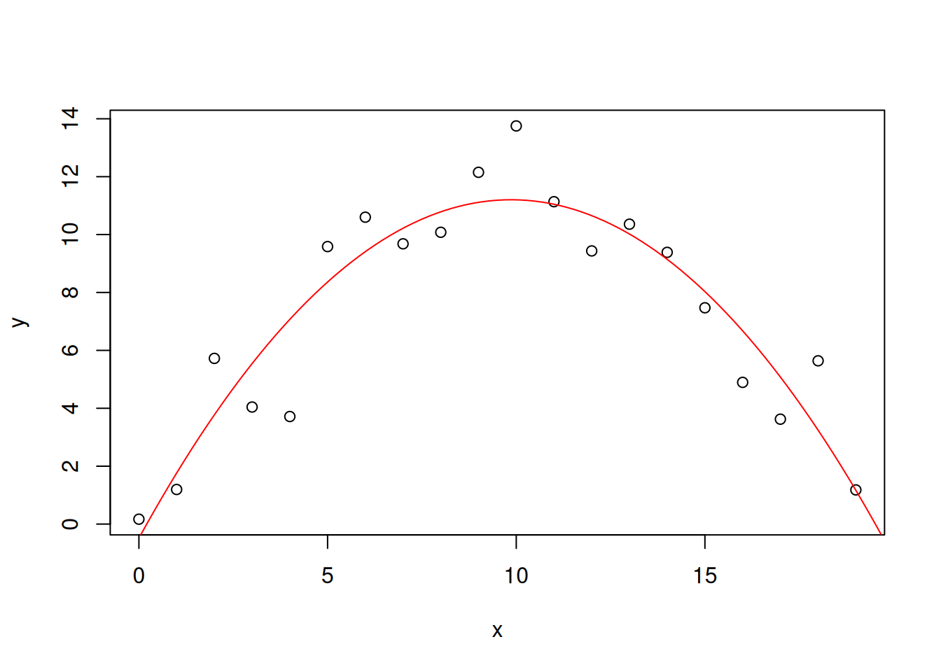
We can check the statistical significance of fitted parameters:
summary(quadmodel)
Call:
lm(formula = y ~ x1 + x2, data = data.frame(x1, x2, y))

Residuals:
    Min      1Q  Median      3Q     Max
-3.3577 -0.8349  0.0507  1.0750  2.5515

Coefficients:
            Estimate Std. Error t value Pr(>|t|)
(Intercept) -0.48599    0.96133  -0.506     0.62
x1           2.37045    0.23452  10.108 1.32e-08 ***
x2          -0.12018    0.01192 -10.086 1.36e-08 ***
---
Signif. codes:  0 '***' 0.001 '**' 0.01 '*' 0.05 '.' 0.1 ' ' 1

Residual standard error: 1.579 on 17 degrees of freedom
Multiple R-squared:  0.8592,    Adjusted R-squared:  0.8427
F-statistic: 51.88 on 2 and 17 DF,  p-value: 5.789e-08
The confidence intervals for estimated parameters:
confint(quadmodel) 2.5 % 97.5 %
(Intercept) -2.5142103 1.54222740
x1 1.8756591 2.86524640
x2 -0.1453202 -0.09504259